Knowing how to create a frequency table is an essential skill when comparing and analyzing data.
As the name suggests, the frequency table lets you see the distribution of values in your data set by showing the number of times each value repeats 🚩
You can use it to quickly identify patterns, and trends and compare frequencies of different types of data. It lets you understand the distribution of values within the data.
In this tutorial, we will see how to make a frequency table and its histogram in Excel. Download our sample workbook here to practice along the guide in real time.
Before we get into making a frequency table using a pivot table, make sure your data set is organized and has no blank cells. That said, let’s get into it 😃
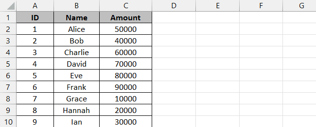
We have the following sample data set we want to create a frequency distribution table out of.
Step 1) Select your data set.
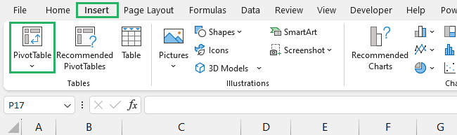
Step 2) Go to the Insert tab and select Pivot Table.
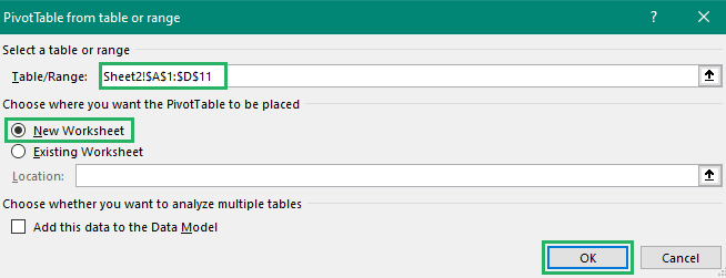
Step 3) The Create Pivot table dialog box will appear.
Step 4) Select a location for your pivot table – we chose a New worksheet.
Step 5) Press Ok.
Step 6) An empty pivot table will appear on the new sheet.
Step 7) Click on the pivot table and a pivot pane will appear on the right side of the screen.
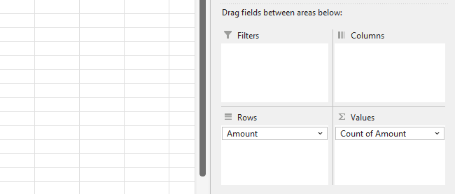
Step 8) Drag the fields you want in the pivot table to the Fields area – we moved Amount to Rows and Values.
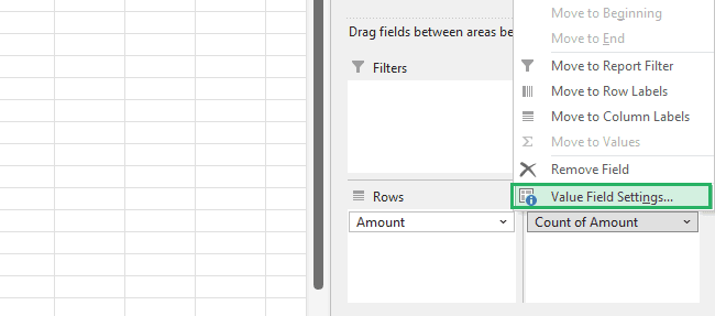
Step 9) Click on the downward arrow next to the field in Values and select Value Field settings.
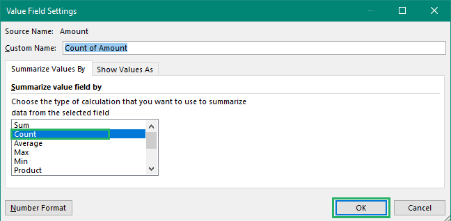
Step 10) A Value Field Settings dialog box will appear.
Step 11) Select Count from the list.
Step 12) Press Ok.
The pivot table will now show the count of each value.
We’ve set the foundation of our table, now for the final string:
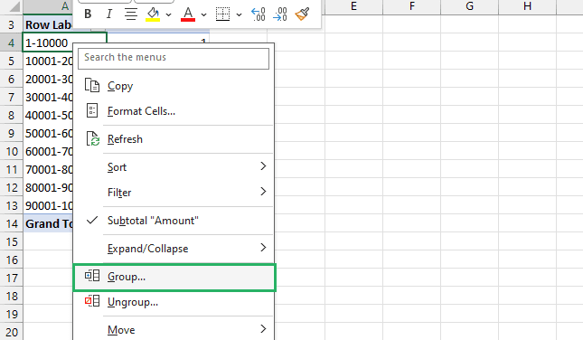
Step 13) Right-click any cell in the Row Labels column.
Step 14) Select Group from the dropdown list.
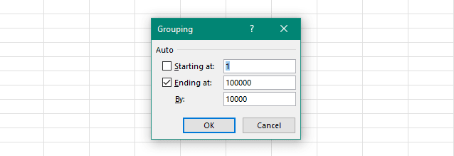
Step 15) Enter the starting, ending and difference values for your data set to group by – we entered 1, 1000 and 10,000, respectively.
Step 16) Press Ok.
And tada! Your frequency pivot table is all done 😀
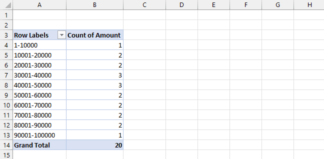
It shows the number of occurrences of each group of values. You can also see the cumulative frequency in the Grand Total row. How cool is that? 🤓
You can create a frequency table manually by sorting and arranging your values but it is quite different than creating a frequency table using a pivot table and requires more effort 🤔
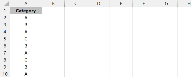
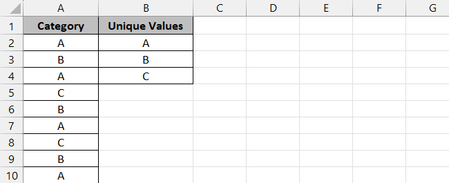
We will use the following sample data with only one column that contains our repetitive values.
To create a frequency distribution table,
Step 1) Create a new helper column and name it Unique Values.
Step 2) Copy the data set and paste it into the Unique Values column.
Step 3) Select the data in the Unique Values column.
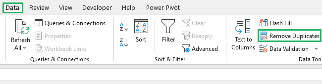
Step 4) Go to the Data tab and select Remove Duplicates from the Data Tools section.
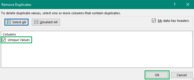
Step 5) The Remove Duplicates dialog box will appear.
Step 6) Make sure only the Unique Values column is selected and check My data has headers option.
Step 7) Press Ok.
Excel will show a prompt, indicating the number of unique values and duplicates found – press Ok.
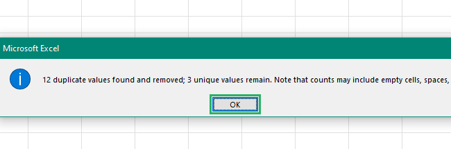
All duplicates will be removed from the Unique Values column and only unique values will be left 🤯
Step 8) Now, create a new frequency column next to the Unique Values column and name it Frequency.
Step 9) In cell C2, type the following formula:
Click to copy Syntax HighlighterStep 10) Press Enter.
Step 11) Double-click the Fill Handle at the bottom right corner of the cell to copy the formula down.
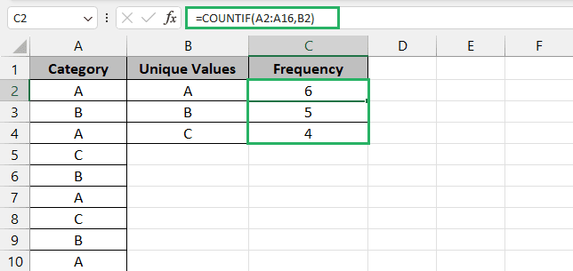
Your frequency distribution table is all ready. You can now use this table to create a histogram to display the data set graphically too 🤠
Once you have all your data in place with a pivot table, now’s the time to create its histogram 📈
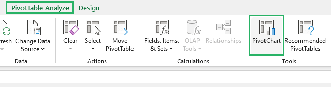
Step 1) Click on the pivot table to activate it.
Step 2) Go to the PivotTable Analyze tab and select Pivot Chart from the Tools section.
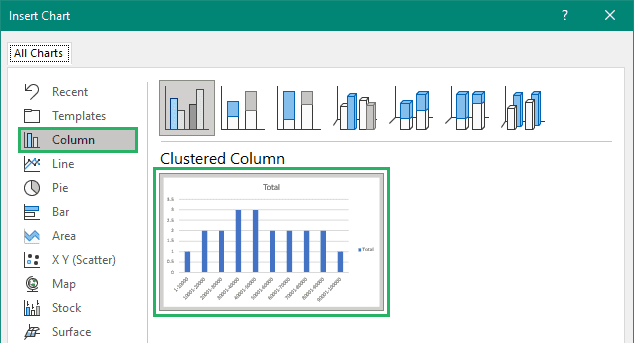
Step 3) The Insert Chart dialog box appears on the screen.
Step 4) Select Clustered Column chart.
Step 5) Press Ok.
And it’s done! The Pivot Chart will appear on the screen as:
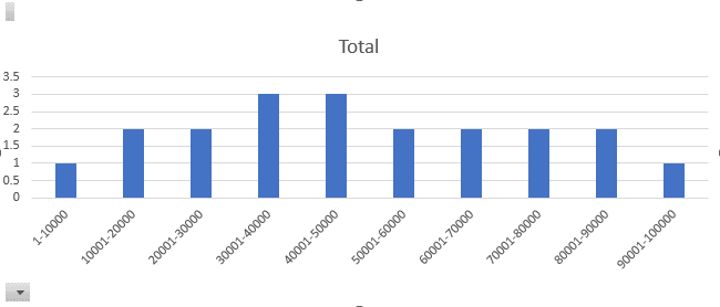
How easy was that? 🧐
Once you have all the data organized and frequency found, creating a histogram for it is very easy. Let’s see how to do it below 🔽
To create a histogram,
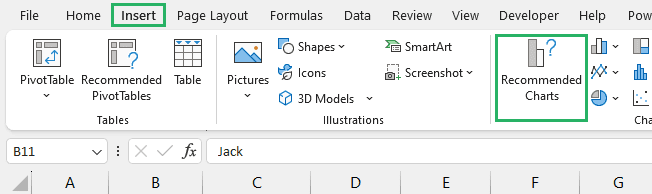
Step 1) Select the unique values and the frequency columns.
Step 2) Go to the Insert tab and click on Recommended Charts.
Step 3) The Recommended Charts dialog box will appear.
Step 4) Select the Clustered Column option.
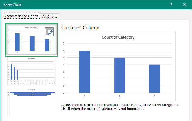
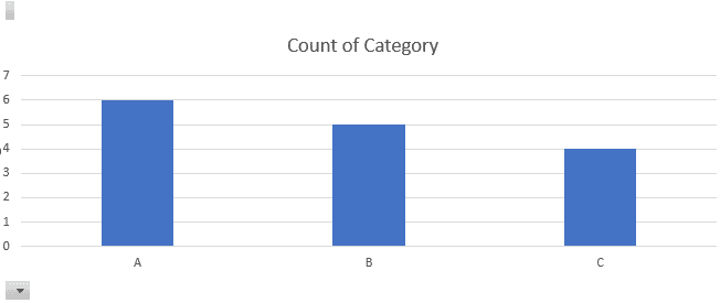
The chart will appear on the screen – you can use this chart if you like.
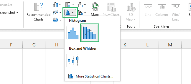
However, if you want to use a Pareto histogram, do this:
Step 5) Click on the chart to activate it.
Step 6) Select Statistical Chart from the Charts section.
Step 7) Select Pareto under Histogram from the dropdown list that appears.
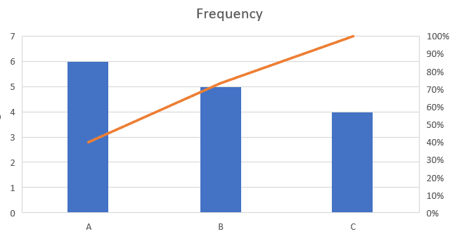
And it’s done! The column chart will be converted to a Pareto Histogram just like that without you having to make data points, input range and other bin adjustments.
If you use directly use a Histogram without this process, it will be very difficult to adjust it. So it’s recommended to follow the above method.
How cool is that? 💪
In this guide, we saw two different ways to create a frequency table in Microsoft Excel. We saw how to do it manually and use a pivot table to do the same
We also learned how to create histograms for the table created in two different ways. A frequency table can be of great help for data analysis where you need to check the frequency of each data set.
It might seem slightly difficult or time-consuming at first, but once you get a hold of its essence, you will be able to do it with your eyes closed.
To learn more about pivot tables, and charts, give the following articles a red.
We hope you enjoyed reading this as much as we enjoyed creating it! 🤗